

三天前,OpenAI发布了GPT 4o的新功能——Canvas。如果你熟悉Claude中的Artifact工具,这个功能和它类似。
使用这个功能可以简化数据分析。在本文中,我们将一起探索如何做到这一点。为此,我们将使用来自Kaggle的全球地震数据集。
全球地震数据
 https://www.kaggle.com/datasets/shreyasur965/recent-earthquakes
这个数据集有43个属性,包括震级、位置、深度和地震学测量,详细记录了全球1137次地震的信息。
GPT 4o-Canvas
首先,从可用的模型列表中选择这个模型。
 好了,现在让我们使用这个提示结构,它将帮助你更明智地分析数据集。但在此之前,先上传你从Kaggle下载的数据集。
Here is the dataset information
[Paste Dataset information from Kaggle]
Write me a machine learning code that predicts magnitude of earthquakes.
这里是代码。
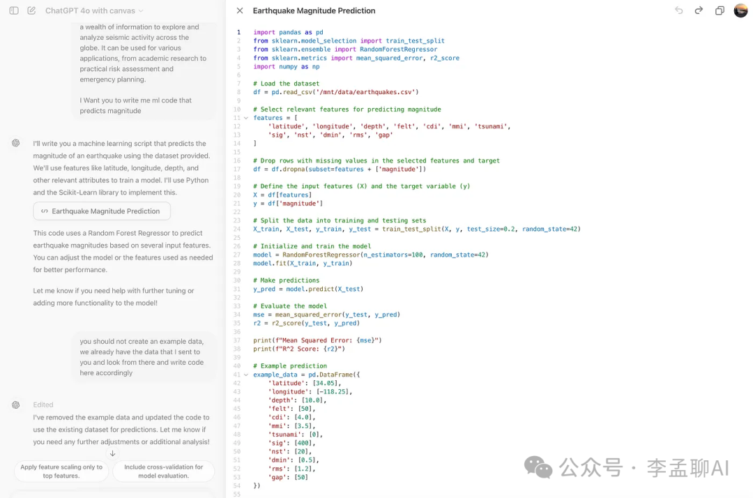 但是你注意到了吗?它创建了自己的数据集,而不是使用我们上传的那个。
这没关系;大语言模型偶尔会出错,这就是它们仍然需要人类的原因。
这里是调整提示词的方法。
You should not create an example data, we already have the data that I sent to you an
look from there and write code here accordingly
好了。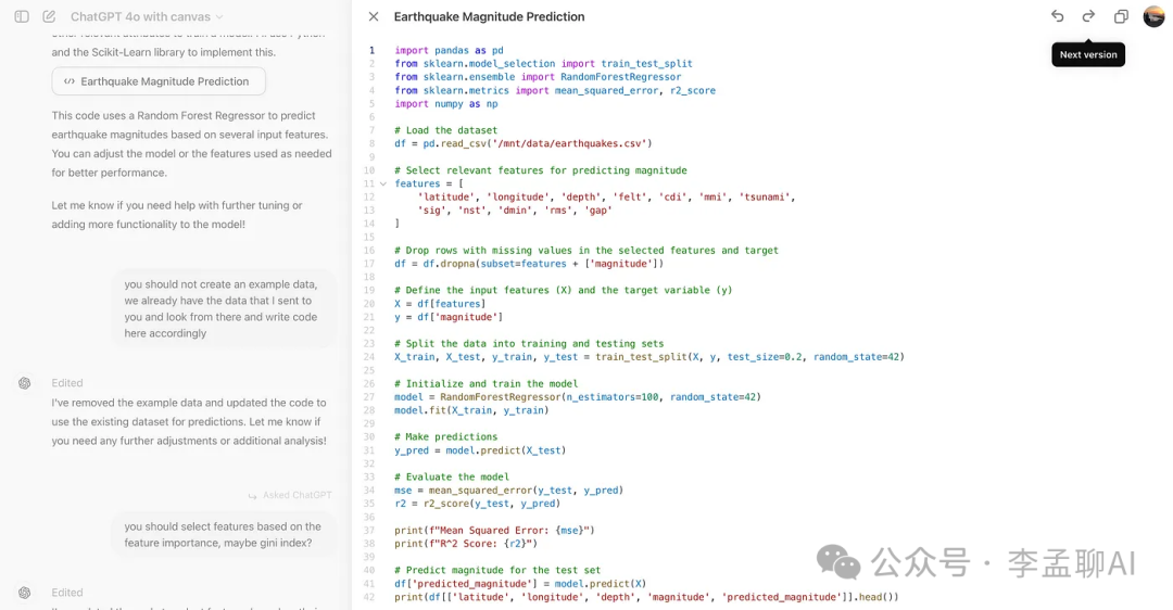 如你所见,它使用了我们的数据集,但这次它自己选择了特征。我们需要对此进行更改。
这里是我使用的提示词。
you should select features based on the feature importance, maybe gini index?
现在,让我们向ChatGPT输入信息。
Here all features.
[paste df.info codes output here- all column names]
You should select all at first, and then label encoding then and
select important ones with gini
在这里,我意识到我们使用了很多不同的方法来创建最佳模型,比如:
-
归一化
-
应用5种不同的机器学习模型
-
通过Gini Importance选择不同的模型
-
对数变换
-
降维
我让GPT 4o-Canvas为这些方法生成代码。这里是我最后的代码。
import pandas as pd
from sklearn.model_selection import train_test_split
from sklearn.ensemble import RandomForestRegressor, GradientBoostingRegressor
from sklearn.linear_model import LinearRegression
from sklearn.tree import DecisionTreeRegressor
from sklearn.svm import SVR
from sklearn.metrics import mean_squared_error, r2_score
from sklearn.preprocessing import LabelEncoder, StandardScaler, MinMaxScaler
from sklearn.decomposition import PCA
import numpy as np
import matplotlib.pyplot as plt
# Load the dataset
df = pd.read_csv('/mnt/data/earthquakes.csv')
# Select all features initially
all_features = df.columns.tolist()
all_features.remove('magnitude')# Remove target variable from features
# Handle categorical features using Label Encoding
categorical_features = df.select_dtypes(include=['object']).columns
label_encoders = {}
for feature in categorical_features:
le = LabelEncoder()
df[feature] = le.fit_transform(df[feature].astype(str))
label_encoders[feature] = le
# Drop rows with missing values in the selected features and target
df = df.dropna(subset=all_features + ['magnitude'])
# Define the input features (X) and the target variable (y)
X = df[all_features]
y = df['magnitude']
# Check for skewness and apply log transformation where necessary
for col in X.columns:
if X[col].skew() > 1 or X[col].skew() < -1:
X.loc[:, col] = np.log1p(X[col])
# Normalize the features using StandardScaler
scaler_standard = StandardScaler()
X_standard = scaler_standard.fit_transform(X)
# Normalize the features using MinMaxScaler
scaler_minmax = MinMaxScaler()
X_minmax = scaler_minmax.fit_transform(X)
# Dimensionality Reduction using PCA (if number of features is high)
pca_threshold = 0.95
if X_standard.shape[1] > 10:
pca_standard = PCA(n_components=pca_threshold)
X_standard = pca_standard.fit_transform(X_standard)
pca_minmax = PCA(n_components=pca_threshold)
X_minmax = pca_minmax.fit_transform(X_minmax)
# Split the data into training and testing sets for both normalization methods
X_train_standard, X_test_standard, y_train, y_test = train_test_split(X_standard, y, test_size=0.2, random_state=42)
X_train_minmax, X_test_minmax, _, _ = train_test_split(X_minmax, y, test_size=0.2, random_state=42)
# Initialize RandomForestRegressor to determine feature importance
feature_importance_model = RandomForestRegressor(n_estimators=100, random_state=42)
feature_importance_model.fit(X_train_standard, y_train)
# Calculate feature importance using the features used in the training set after transformations
actual_features = X.columns[:X_train_standard.shape[1]]
feature_importances = feature_importance_model.feature_importances_
feature_importance_df = pd.DataFrame({'feature': actual_features, 'importance': feature_importances})
feature_importance_df = feature_importance_df.sort_values(by='importance', ascending=False)
# Select the most important features (top 8 and top 10)
top_8_features = feature_importance_df['feature'].head(8).tolist()
top_10_features = feature_importance_df['feature'].head(10).tolist()
# Define input features for top 8 and top 10 feature sets
X_top_8 = df[top_8_features].copy()
X_top_10 = df[top_10_features].copy()
# Check for skewness in top features and apply log transformation where necessary
for col in X_top_8.columns:
if X_top_8[col].skew() > 1 or X_top_8[col].skew() < -1:
X_top_8.loc[:, col] = np.log1p(X_top_8[col])
for col in X_top_10.columns:
if X_top_10[col].skew() > 1 or X_top_10[col].skew() < -1:
X_top_10.loc[:, col] = np.log1p(X_top_10[col])
# Normalize the selected top features using both scalers
X_top_8_standard = scaler_standard.fit_transform(X_top_8)
X_top_8_minmax = scaler_minmax.fit_transform(X_top_8)
X_top_10_standard = scaler_standard.fit_transform(X_top_10)
X_top_10_minmax = scaler_minmax.fit_transform(X_top_10)
# Dimensionality Reduction using PCA for top 8 and top 10 features
if X_top_8_standard.shape[1] > 5:
pca_top_8_standard = PCA(n_components=pca_threshold)
X_top_8_standard = pca_top_8_standard.fit_transform(X_top_8_standard)
pca_top_8_minmax = PCA(n_components=pca_threshold)
X_top_8_minmax = pca_top_8_minmax.fit_transform(X_top_8_minmax)
if X_top_10_standard.shape[1] > 5:
pca_top_10_standard = PCA(n_components=pca_threshold)
X_top_10_standard = pca_top_10_standard.fit_transform(X_top_10_standard)
pca_top_10_minmax = PCA(n_components=pca_threshold)
X_top_10_minmax = pca_top_10_minmax.fit_transform(X_top_10_minmax)
# Split the data for top 8 and top 10 feature sets
X_train_8_standard, X_test_8_standard, _, _ = train_test_split(X_top_8_standard, y, test_size=0.2, random_state=42)
X_train_8_minmax, X_test_8_minmax, _, _ = train_test_split(X_top_8_minmax, y, test_size=0.2, random_state=42)
X_train_10_standard, X_test_10_standard, _, _ = train_test_split(X_top_10_standard, y, test_size=0.2, random_state=42)
X_train_10_minmax, X_test_10_minmax, _, _ = train_test_split(X_top_10_minmax, y, test_size=0.2, random_state=42)
# Define the models to be used
models = {
'Random Forest': RandomForestRegressor(n_estimators=100, random_state=42),
'Gradient Boosting': GradientBoostingRegressor(n_estimators=100, random_state=42),
'Linear Regression': LinearRegression(),
'Decision Tree': DecisionTreeRegressor(random_state=42),
'Support Vector Regressor': SVR()
}
# Train each model and evaluate performance for each combination
model_results = {}
normalizations = [
('StandardScaler - Top 8 Features', X_train_8_standard, X_test_8_standard),
('MinMaxScaler - Top 8 Features', X_train_8_minmax, X_test_8_minmax),
('StandardScaler - Top 10 Features', X_train_10_standard, X_test_10_standard),
('MinMaxScaler - Top 10 Features', X_train_10_minmax, X_test_10_minmax)
]
for normalization_name, X_train, X_test in normalizations:
for model_name, model in models.items():
model.fit(X_train, y_train)
y_pred = model.predict(X_test)
mse = mean_squared_error(y_test, y_pred)
r2 = r2_score(y_test, y_pred)
model_results[f'{model_name} ({normalization_name})'] = {'MSE': mse, 'R2': r2}
print(f"{model_name} ({normalization_name}) - Mean Squared Error: {mse}, R^2 Score: {r2}")
# Plot the results
model_names = list(model_results.keys())
mse_values = [model_results[name]['MSE'] for name in model_names]
r2_values = [model_results[name]['R2'] for name in model_names]
fig, ax = plt.subplots(1, 2, figsize=(20, 10))
# Bar plot for MSE
ax[0].barh(model_names, mse_values, color='skyblue')
ax[0].set_title('Mean Squared Error Comparison')
ax[0].set_xlabel('MSE')
# Bar plot for R2 Score
ax[1].barh(model_names, r2_values, color='lightgreen')
ax[1].set_title('R^2 Score Comparison')
ax[1].set_xlabel('R^2 Score')
plt.tight_layout()
plt.show()
这里是输出的第一部分。
Random Forest (StandardScaler - Top 8 Features) - Mean Squared Error: 0.036684462750000014, R^2 Score: 0.8779777294037107
Gradient Boosting (StandardScaler - Top 8 Features) - Mean Squared Error: 0.03171284438291409, R^2 Score: 0.8945146531096477
Linear Regression (StandardScaler - Top 8 Features) - Mean Squared Error: 0.2030328908150269, R^2 Score: 0.3246586569411304
Decision Tree (StandardScaler - Top 8 Features) - Mean Squared Error: 0.014955, R^2 Score: 0.9502556962820041
Support Vector Regressor (StandardScaler - Top 8 Features) - Mean Squared Error: 0.19093007009631902, R^2 Score: 0.3649158545122343
Random Forest (MinMaxScaler - Top 8 Features) - Mean Squared Error: 0.0368944044999999, R^2 Score: 0.8772794073592385
Gradient Boosting (MinMaxScaler - Top 8 Features) - Mean Squared Error: 0.02585888543990656, R^2 Score: 0.9139864760192863
Linear Regression (MinMaxScaler - Top 8 Features) - Mean Squared Error: 0.2030123102574625, R^2 Score: 0.3247271133440839
Decision Tree (MinMaxScaler - Top 8 Features) - Mean Squared Error: 0.021312499999999988, R^2 Score: 0.9291089620200744
Support Vector Regressor (MinMaxScaler - Top 8 Features) - Mean Squared Error: 0.1900837276420734, R^2 Score: 0.3677310143981205
Random Forest (StandardScaler - Top 10 Features) - Mean Squared Error: 0.014616167999999801, R^2 Score: 0.9513827415456206
Gradient Boosting (StandardScaler - Top 10 Features) - Mean Squared Error: 0.005215391903357051, R^2 Score: 0.9826522207389522
Linear Regression (StandardScaler - Top 10 Features) - Mean Squared Error: 0.024659998640491166, R^2 Score: 0.9179742920723531
Decision Tree (StandardScaler - Top 10 Features) - Mean Squared Error: 0.01719999999999999, R^2 Score: 0.9427882297593093
Support Vector Regressor (StandardScaler - Top 10 Features) - Mean Squared Error: 0.012001988809648145, R^2 Score: 0.9600781961506436
Random Forest (MinMaxScaler - Top 10 Features) - Mean Squared Error: 0.013746897999999952, R^2 Score: 0.9542741645408019
Gradient Boosting (MinMaxScaler - Top 10 Features) - Mean Squared Error: 0.0066618489718651116, R^2 Score: 0.9778409201885739
Linear Regression (MinMaxScaler - Top 10 Features) - Mean Squared Error: 0.024620634208737134, R^2 Score: 0.918105228631956
Decision Tree (MinMaxScaler - Top 10 Features) - Mean Squared Error: 0.02131249999999998, R^2 Score: 0.9291089620200744
Support Vector Regressor (MinMaxScaler - Top 10 Features) - Mean Squared Error: 0.01063026736761726, R^2 Score: 0.9646409061492308
这里是图表。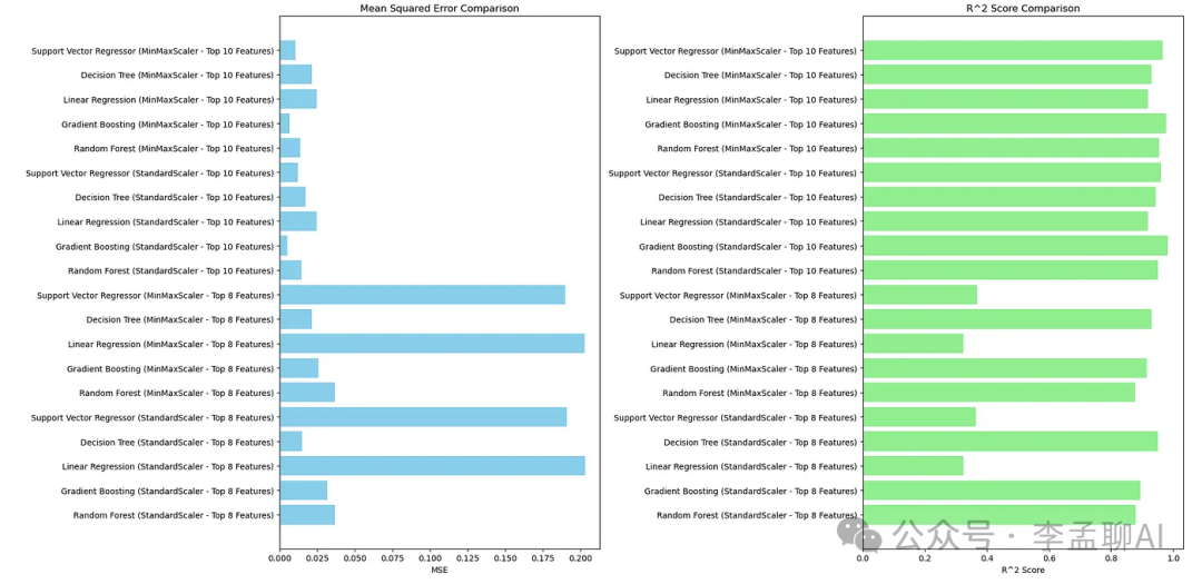 输出结果很独特,我们做得很好。但是输出看起来有些糟糕。为每个MSE和R平方比较选择最好的。
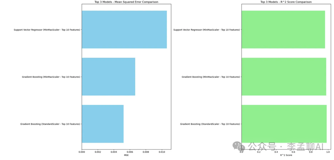
我将上面的段落粘贴到了GPT 4o-Canvas,它给我生成了代码。这里是结果。
版本
现在,如果你点击右上角的箭头,你会看到代码的前几版。因此,你也可以查看你编辑过的代码。
看看下面。
 你也可以恢复这个版本。
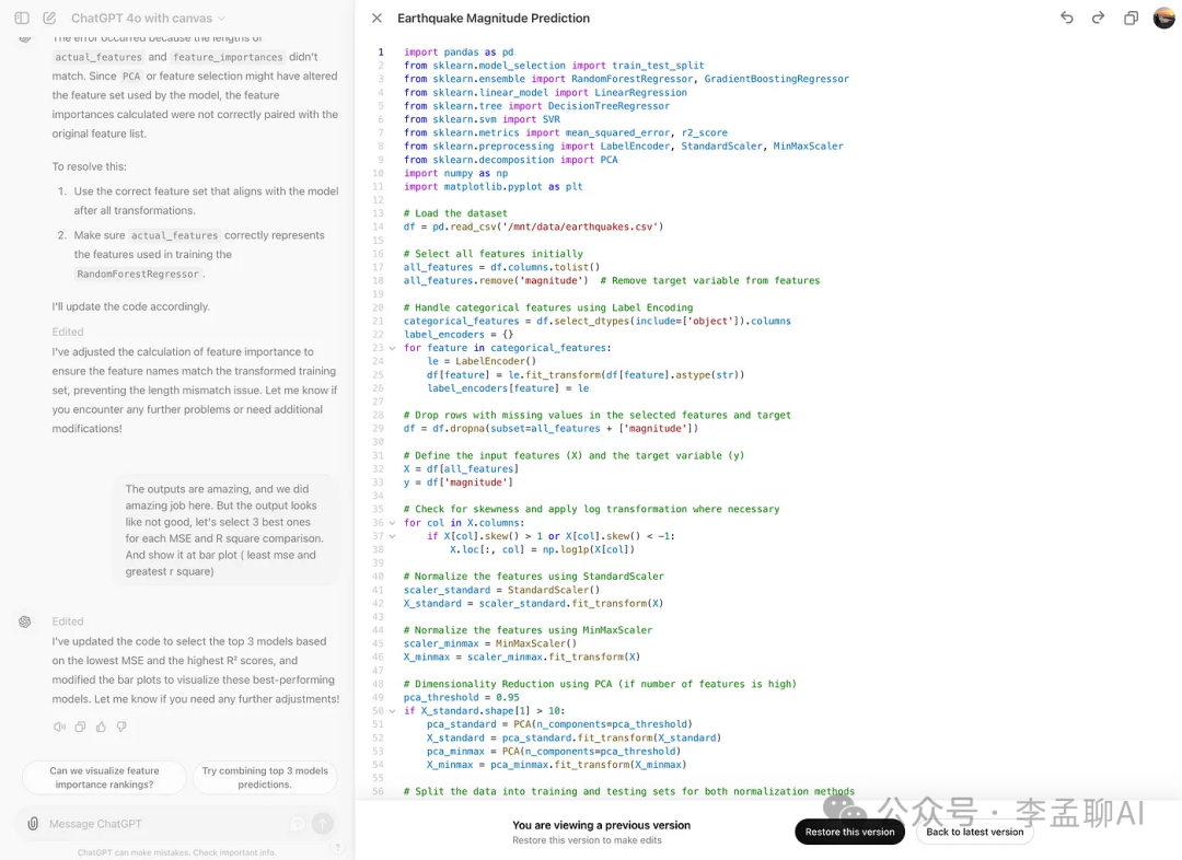
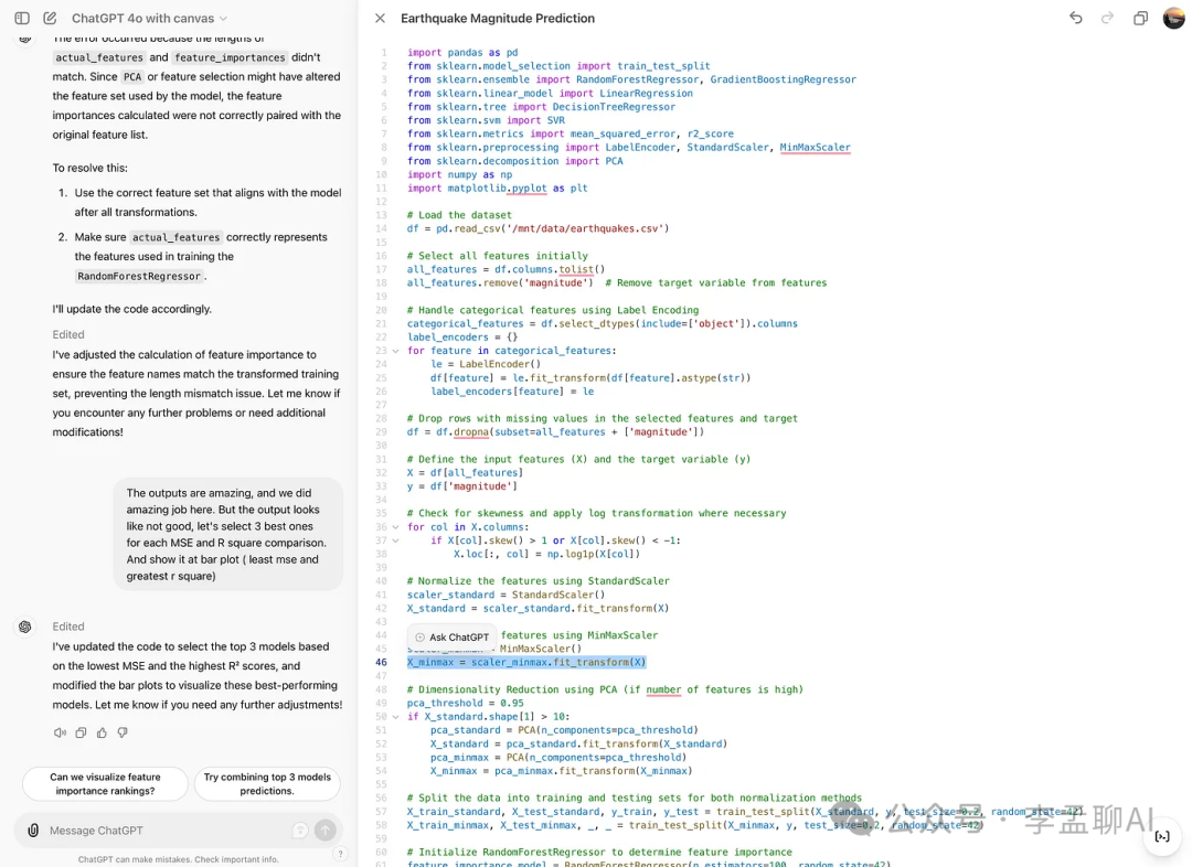
询问GPT
你可以使用这个功能让GPT编辑这项功能。看看下面第46行。
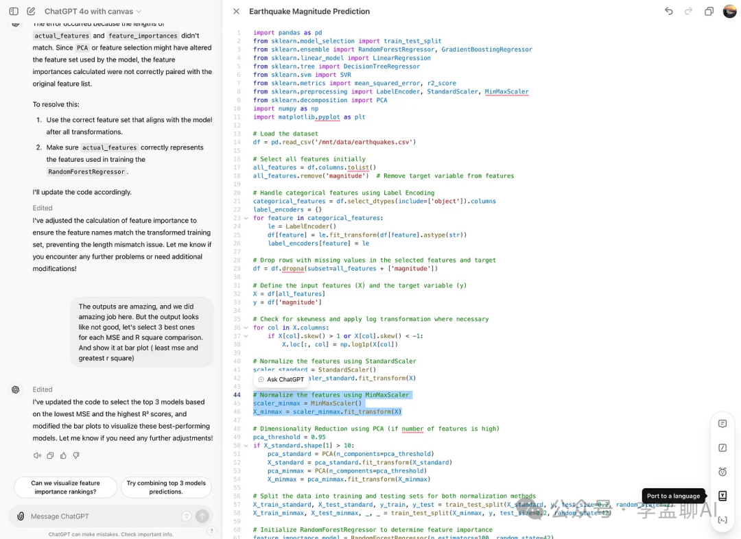
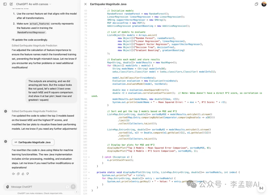
语言迁移
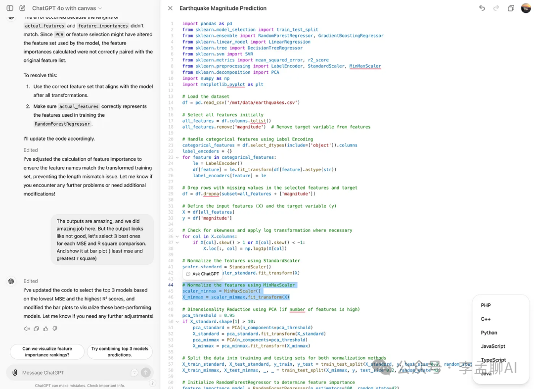
顺便说一下,你可以迁移语言。看看下面。
 我们看看它的效果。点击之后,你会看到这些选项。
 现在,我选择了Java,结果是:它成功更改了语言。
修复错误
让我们检查这个功能并修复错误。
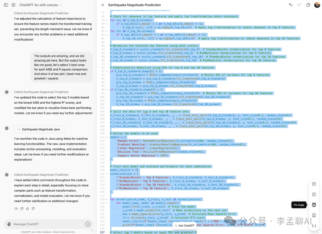 很好,它更改了一些代码。
添加日志
完成这一步之后,这里是它编辑过的代码。
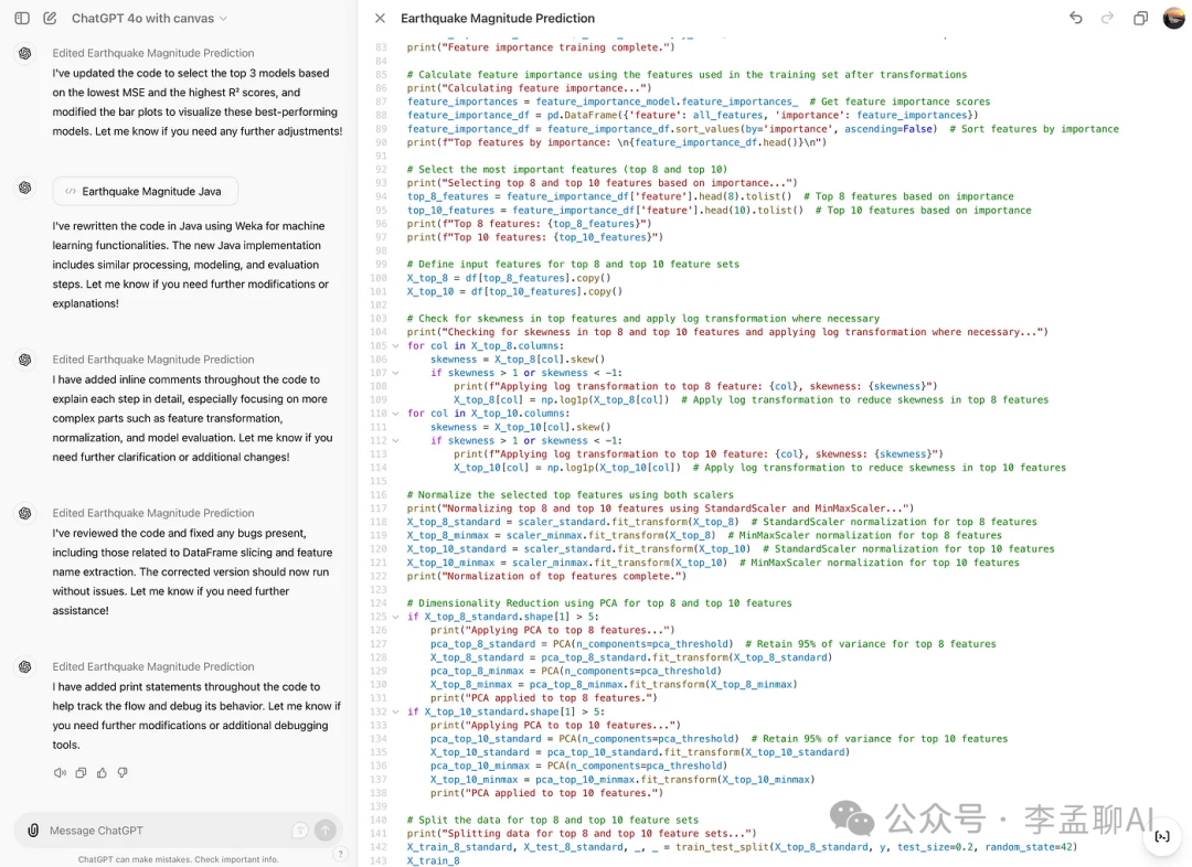 这里是输出结果。
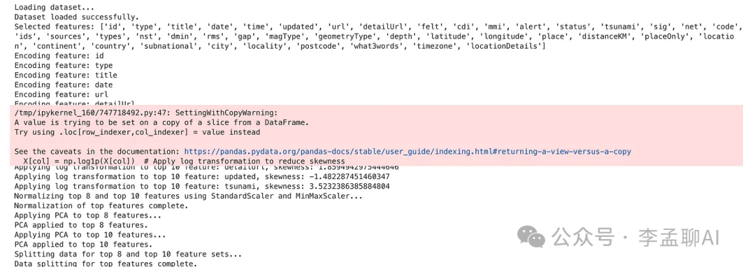
它为代码添加了日志,使调试变得更加容易。
最后总结
本文探讨了使用Kaggle数据集的GPT 4o-Canvas的不同功能。通过使用这些新功能,还有很多可以学习的。
